Data Preprocessing for Machine Learning

In this guide, we will learn how to do data preprocessing for machine learning.
Data Preprocessing is a very vital step in Machine Learning. Most of the real-world data that we get is messy, so we need to clean this data before feeding it into our Machine Learning Model. This process is called Data Preprocessing or Data Cleaning. At the end of this guide, you will be able to clean your datasets before training a machine learning model with it.

Prerequisites:

• A laptop
• Jupyter Notebook
• Basic Python Programming knowledge
• Sample Dataset (click here to download)

I will be using Jupyter Notebook. To get Jupyter Notebook, you need to install Anaconda. You can follow this tutorial video on how to install Anaconda by clicking here.

In this article, I will cover the following:

• Importing libraries
• Importing dataset
• Handling Duplicate Values
• Handling Missing values
• Encoding Categorical data
• Splitting the dataset
• Feature Scaling

Importing Libraries
The basic libraries that we will be using are NumPy, pandas, matplotlib, and sklearn.

# importing libraries
import numpy as np
import matplotlib.pyplot as plt
import pandas as pd

We will use the Pandas library to import our dataset and do some data analysis. The NumPy library helps us work with arrays. Our data must be converted to a NumPy array before training. The Matplotlib library will help us with data visualization.

Importing the Dataset
We will use the Pandas library to import our dataset, which is a CSV file. CSV stands for Comma-Separated Values.

# import dataset
dataset = pd.read_csv('sample_data.csv')
print(dataset)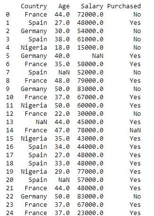

Let’s view some rows of our dataset

# viewing the first few rows of the dataset
dataset.head()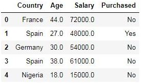

We can also view statistical information about our dataset by using the .describe() method.

# viewing statistical info about dataset
dataset.describe()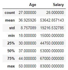

Removing Duplicate Values
Sometimes our dataset may contain duplicate values. These duplicate values are not necessary, so we need to remove them.

# dropping duplicate values
dataset = dataset.drop_duplicates()
print(dataset)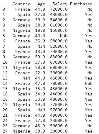

We can run the .describe() method on our dataset to check if there are any changes

dataset.describe()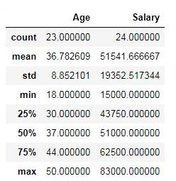

Handling Missing Data
In our dataset, there may be some missing values. We cannot train our model with a dataset that contains missing values. So we have to check if our dataset has missing values.

# checking for missing values
dataset.isnull()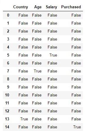

# checking the number of missing data
dataset.isnull().sum()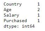

We can handle missing values by:

Deleting the row/column: This is one of the easiest ways to handle missing values. If we have a lot of missing values in a column, we can just remove that column from our dataset. We could also delete any row with missing values. The only problem with this method is that we lose some information needed by our model to make accurate predictions.

Replacing missing values with Mean/Mode/Median: For numerical data, we can replace missing values with the mean, mode, or median of the column with the missing value. This way we get to preserve some information needed by our model. The mean is mostly preferred.

Replacing with values close to the missing value: We could also replace missing values with the value that comes before or after it in the same column.

For the columns ‘Country’ and ‘Purchased’, I will remove the rows with missing values.

# Dropping categorical data rows with missing values
dataset.dropna(how='any', subset=['Country', 'Purchased'], inplace=True)

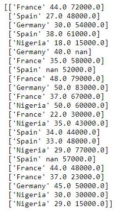
Before I replace the missing values in the other columns, I will separate the independent variables and target variable. The target variable is what we are trying to predict. While the independent variables are the features that will help us make the predictions. The columns ‘Country’, ‘Age’, and ‘Salary’ are our independent variables, while ‘Purchased’ is our target variable.

In the code above, for the parameter ‘how’, the argument ‘any’ drops the row if any value is null. But the argument ‘all’ will only drop the row if all the values are null. The argument for the ‘subset’ parameter is a list containing the columns we want to remove missing values from. ‘inplace=True’ modifies our original dataframe, instead of returning a copy of the dataframe.

# Splitting dataset into independent & dependent variable
X = dataset[['Country', 'Age', 'Salary']].values
y = dataset['Purchased'].values
print(X)

Note that ‘.values’ will convert our dataframe to a numpy array.

print(y)

We will replace the missing values in the ‘Age’ and ‘Salary’ columns with the mean.

# replacing the missing values in the age & salary column with the mean
# import the SimpleImputer class from the sklearn library
from sklearn.impute import SimpleImputer
print(X[:, 1:3])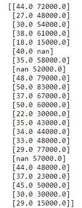

imputer = SimpleImputer(missing_values=np.nan, strategy='mean')
imputer.fit(X[:, 1:3])
X[:, 1:3] = imputer.transform(X[:, 1:3])
print(X[:, 1:3])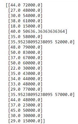

In the SimpleImputer() class, np.nan represents the missing values in our NumPy array. That will be the argument to the ‘missing_values’ parameter. ‘strategy=mean’ means we will be replacing the missing values with the mean.

The .fit() method will connect our ‘imputer’ object to the matrix of features X. But to do the replacement, we need to call another method, this is the .transform() method. This will apply the transformation, thereby replacing the missing values with the mean.

Encoding Categorical Data
Deborah Rumsey defines categorical data as the type of data that is used to group information with similar characteristics. In our dataset, the ‘Country’ & ‘Purchased’ columns contain categorical data.

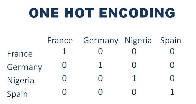
Our Machine Learning Model works with numbers, so our model won’t understand these categorical data. We need to encode these categorical data into numbers. To do this, we apply One-Hot Encoding. One Hot Encoding converts the column with the categorical data into multiple new columns as shown below:

From sklearn.compose, we will import the ColumnTransformer class. We will also import OneHotEncoder class from the preprocessing module of the sklearn library.

# Handling Categorical Data
from sklearn.compose import ColumnTransformer
from sklearn.preprocessing import OneHotEncoder

ct = ColumnTransformer(transformers=[('enconder', OneHotEncoder(), [0])], remainder='passthrough')
X = np.array(ct.fit_transform(X))
print(X)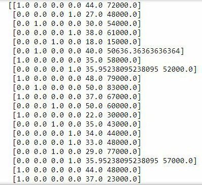

In the ColumnTransformer class, for the argument ‘transformers’, we have a list containing a tuple as the parameter. The first item ‘encoder’ is the type of transformation we want. ‘OneHotEncoder()’ is the class that will handle the transformation. ‘[0]’ is the index of the column we want to encode. If we have multiple columns to transform, we can put them in the list. In this case, we only have one column with index 0, so it is only 0 that is in the list. The remainder=’passthrough’ means we want to leave the other columns the way they are without transforming them.

print(y)

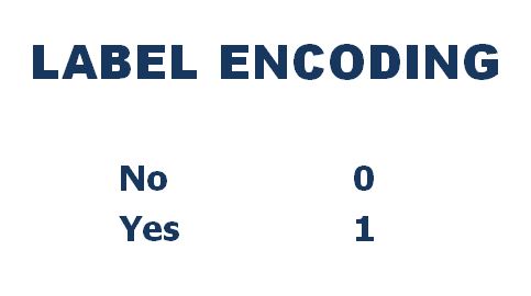
For our target variable ‘Purchased’, we will apply Label Encoding instead of One Hot Encoding. This is because we need No to be represented by 0 and Yes to be represented by 1.

# Encoding the target variable
from sklearn.preprocessing import LabelEncoder
le = LabelEncoder()
y = le.fit_transform(y)
print(y)

Splitting the Dataset
Splitting our dataset into training & test set is another important step in data preprocessing. We will use part of the dataset to train the model. The other part of the dataset will be used to evaluate our model, to see how it performs on new data that it hasn’t seen before. We will do the split in the 80:20 ratio. 80% of the dataset will be used for training, while 20% will be used for testing.

# Splitting Dataset into Training and Test Set
from sklearn.model_selection import train_test_split
X_train, X_test, y_train, y_test = train_test_split(X, y, test_size=0.2                                                , random_state=2)

For the train_test_split function, the argument X is our features (independent variable). The argument y is our target variable,
‘test_size=0.2’ means 20% of the dataset will be used as the test set. The random_state sets a seed to the random generator.

print(X_train)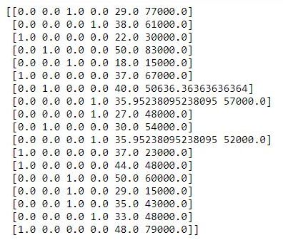

print(X_test)

print(y_train)

print(y_test)

Feature Scaling
This is the final step of data preprocessing. Feature scaling puts all our data in the same range and on the same scale. We do not want any feature of our dataset to dominate another feature. We don’t have to apply feature scaling to all datasets, especially if the features of that dataset are already within the same range. We could apply normalization or standardization to our dataset. The formula is shown below:

Standardization puts all the values between the range of -3 and 3. But normalization will always give you positive values between the range of 0 and 1.
We will apply standardization. We will use the StandardScaler class from the preprocessing module of the sklearn library. We won’t apply feature scaling to the one-hot encoded columns (dummy variables). We don’t want to change the interpretation of those values.

# Feature Scaling
from sklearn.preprocessing import StandardScaler
sc = StandardScaler()
X_train[:, 4:] = sc.fit_transform(X_train[:, 4:])

The .fit() method of the StandardScaler() class will just calculate the mean and standard deviation for X_train, while the .transform() method will transform the values with the formula above. We can do the fit and transform in one line of code by using the .fit_transform() method.

print(X_train)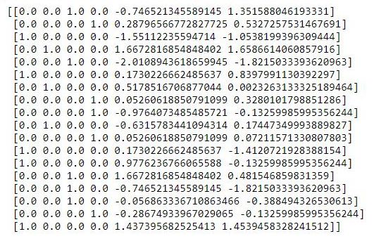

print(X_test)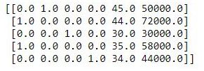

X_test[:, 4:] = sc.transform(X_test[:, 4:])
print(X_test)

Conclusion

Before we can train a Machine Learning model, we need to clean our data.
If we don’t clean our dataset, we will run into some problems during training. We need to handle missing values, encode categorical variables, and sometimes apply feature scaling to our dataset.

After data preprocessing, we can now train our machine learning model.

Check out the Github repo here.