Building a Simple Linear Regression Model with Sci-kit Learn

In this guide, we will learn how to build a Simple Linear Regression Model using Sci-kit Learn. Simple Linear Regression is a regression algorithm that shows the relationship between a single independent variable and a dependent variable.
The Sci-kit Learn library contains a lot of tools used for machine learning. We will build a model to predict sales revenue from the advertising dataset using simple linear regression.

Prerequisite

• A PC with Jupyter Notebook IDE
• Advertising dataset from Kaggle

The formula of simple linear regression is:

            y = θ0x + θ1

θ0 represents the slope of the regression line
θ1 represents the intercept of the regression line
x is the independent variable
y is the dependent variable

IMPORTING DATASET
Let’s import our libraries

# importing libraries
import pandas as pd
import numpy as np
from matplotlib import pyplot as plt
%matplotlib inline



# importing dataset
advert = pd.read_csv('Advertising.csv')
# view first 5 entries
advert.head()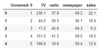

# viewing rows and columns details
advert.info()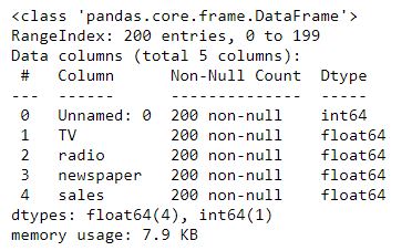

We’ve created a pandas dataframe with 5 columns and 200 rows.
Let’s view our column names.

# getting columns in dataset
advert.columns

There’s a column with the name ‘Unnamed: 0’. That is our index column and we don’t need it, so we will get rid of it using the drop() method from pandas.

# Removing the index column
advert.drop(['Unnamed: 0'], axis=1, inplace=True)

The first argument in the drop method is a list containing the column we want to drop. We set the axis parameter to 1, since we are dropping a column, and the inplace parameter is to True, to modify the original dataframe instead of creating a copy of the dataframe with the ‘Unnamed: 0’ column removed.
Now we can view our dataset again to see if the changes have been implemented.

advert.head()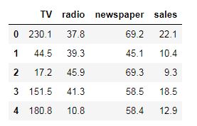

EXPLORATORY DATA ANALYSIS
Let’s do some exploratory data analysis. We will import the Seaborn library.
The Seaborn library is used for data visualization. We will check which feature has the most impact to our sales revenue. We will use the pairplot() method from seaborn to do this.

# Exploratory Data Analysis
import seaborn as sns
# Exploring relationship between Features and Response
sns.pairplot(advert, x_vars=['TV', 'radio', 'newspaper'],
             y_vars='sales', height=10, aspect=0.7, kind='reg')

The first argument in the pairplot() method is our dataframe ‘advert’, the second argument is a list of our features under the x_vars parameter, the third argument is sales under the parameter y_vars. The fourth parameter is the height which is set to 10. The aspect parameter allows us to control the size of our graph. Using the parameter kind, we will specify the kind of pair plot we want. We set it to reg to plot a linear regression on the graph.

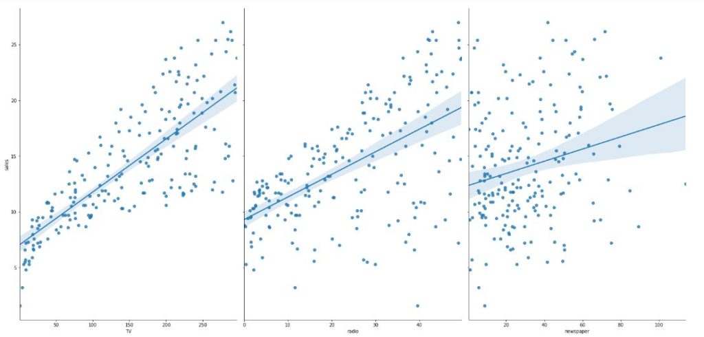
Looking at the graph, we notice that there’s a strong relationship between TV and Sales, but there’s a weak relationship between Radio and Sales. There is an extremely weak relationship between Newspaper and Sales. Let’s check the Pearson correlation between TV and Sales.

# checking Pearson correlation between TV and sales
advert.TV.corr(advert.sales)

We get approximately 0.78, which indicates a very high positive correlation.
We can also check the pairwise correlation of all the columns using the corr() method.

# checking correlation of all columns
advert.corr()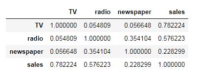

We can also use the heatmap() method of seaborn to view the heatmap correlation matrix.

# Visualizing correlation using seaborn heatmap
sns.heatmap(advert.corr(), annot=True)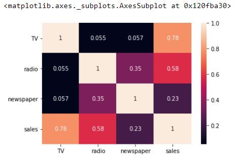

Setting the annot parameter to True will display the correlation coefficients.

So we will use just the TV feature to build our simple linear regression model since it has the highest correlation with Sales.

CREATING THE SIMPLE LINEAR REGRESSION MODEL
We will extract our feature and our target variable. Remember, simple linear regression uses only one feature and that feature will be TV.

# Creating a Simple Linear Regression Model
# using TV and sales only
X = advert[['TV']]
X.head()

# checking the no of rows and columns we are dealing with
print(X.shape)

# Setting target variable/response
y = advert.sales
print(y.shape)

# Splitting Dataset into Train & Test Set
from sklearn.model_selection import train_test_split
X_train, X_test, y_train, y_test = train_test_split(X, y,
                                                    random_state=1)

We will check the shape of X_train, y_train, X_test and y_test.

print(X_train.shape)

print(y_train.shape)

print(X_test.shape)

print(y_test.shape)

By default, 25% of our data will be used as the test set. So out of 200 records, 150 will be used for training and the remaining 50 will be used for testing. Note that sklearn expects our feature matrix, x, to be a numpy array.

from sklearn.linear_model import LinearRegression
linreg = LinearRegression()
linreg.fit(X_train, y_train)

We will import the LinearRegression class from the linear_model module of the Sklearn library. We will create an object of the LinearRegression class and fit it to our training data using the fit() method. Note that Sklearn expects our feature matrix, x, to be a Numpy array.

Now that our model has been fitted to the training set, we can view the model’s coefficient and intercept value.

# Interpreting Model Coefficients
print(linreg.coef_)  # model coefficient value
print(linreg.intercept_)  # model intercept value

Our slope value, θ0 is 0.04802945 and our intercept value, θ1 is 6.91197261886872

MAKING NEW PREDICTIONS WITH THE MODEL
We will now evaluate our model on the test set. The test set is data our model hasn’t seen before.

# Making Predictions with Model
y_pred = linreg.predict(X_test)



# viewing the first 5 predictions
y_pred[:5]

EVALUATING THE MODEL
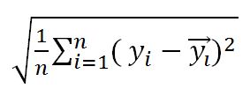
We can evaluate Regression Models by using Mean Absolute Error (MAE), Mean Squared Error (MSE), and Root Mean Squared Error (RMSE).

Mean Absolute Error (MAE)

yi is the actual value of sales while
yi_bar is the predicted value
n is the number of data

Mean Squared Error (MSE)

Root Mean Squared Error (RMSE)

# Model Evaluation
from sklearn import metrics

# Mean Absolute Error
print(metrics.mean_absolute_error(y_test, y_pred))

# Mean Squared Error
print(metrics.mean_squared_error(y_test, y_pred))

# Root Mean Squared Error
print(np.sqrt(metrics.mean_squared_error(y_test, y_pred)))

CONCLUSION
In this guide, we learned how to build a Simple Linear Regression Model using Sci-kit Learn. We were able to fit the model to our training set and make new predictions with our test set. We were also able to evaluate our model using Mean Absolute Error, Mean Squared Error, and Root Mean Squared Error.

In most real-life problems, it takes more than one feature to make an accurate prediction. For example, in trying to predict the price of a house, we cannot use a single feature like the size of the house. We need to consider other features like the number of rooms, location of the house, etc. This is where Multiple Linear Regression comes in.

The Github repo is here.